Geometry Representations
This section describes the geometry representations of the data structures defined in ProGeomitem.h. These structures are output by the geometry functions described in detail in the Core: 3D Geometry section.
Domain of Evaluation
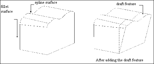
Surfaces and edges can be extended from their original domain as the user continues to add features to the model. For example, the user can add a feature such as a draft surface or local push, which requires the original surface to be extended outside its original domain.
When this occurs, you will find that the uv parameters of the surface have been extended. The ProSurfacedata data structure reflects the extension, and returns the updated values for the u and v extents.
Because the evaluator functions use the analytical surface (or curve) definition, they work for any parameter values. Thus, any surface (or curve) can be extended as needed. In addition, if you pass in parameters outside the current uv domain, the evaluator functions still return values for the parameters as requested.
If you are using the evaluators supplied by Creo TOOLKIT, you do not have to do anything. For surfaces, the evaluator functions work over this extended range of parameters. Your evaluator function for foreign datum surfaces is also expected to allow for extrapolation.
Edges are always parameterized between 0.0 and 1.0. When surfaces are extended, new edges are created that have parameters in the range 0.0 to 1.0.
If you develop your own evaluator functions, you must be aware that the domain of a surface can be extended, as with foreign datum surfaces.
Surfaces
Image
Surface Data Structures
The surface structure contains data that describes the boundary of the surface, and a pointer to the primitive surface on which it lies. The primitive surface is a three-dimensional geometric surface parameterized by two variables (u and v). The surface boundary consists of closed loops (contours) of edges. Each edge is attached to two surfaces, and each edge contains the u and v values of the portion of the boundary that it forms for both surfaces. Surface boundaries are traversed clockwise around the outside of a surface, so an edge has a direction in each surface with respect to the direction of traversal.
Other data found in the surface structure includes the rectangular extents of the two-dimensional domain, the three-dimensional surface, and a flag indicating whether the surface normal points towards the inside or outside of the part. The user data is intended for run-time use only, and this information is not stored with the surface.
This section describes the surface data structures. The data structures are listed in order of complexity. For ease of use, the alphabetical listing of the data structures is as follows:
Plane
Plane
Image
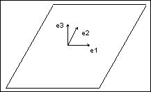
The plane entity consists of two perpendicular unit vectors (e1 and e2), the normal to the plane (e3), and the origin of the plane.
Data Format:
e1[3]       Unit vector, in the u direction
e2[3]       Unit vector, in the v direction
e3[3]       Normal to the plane
origin[3]   Origin of the plane
Parameterization:
(x, y, z) = u * e1 + v * e2 + origin
Cylinder
Cylinder
Image
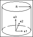
The generating curve of a cylinder is a line, parallel to the axis, at a distance R from the axis. The radial distance of a point is constant, and the height of the point isv.
Data Format:
e1[3]       Unit vector, in the u direction
e2[3]       Unit vector, in the v direction
e3[3]       Normal to the plane
origin[3]   Origin of the plane
radius      Radius of the cylinder
Parameterization:
(x, y, z) = radius * [cos(u) * e1 + sin(u) * e2] +
           v * e3 + origin
Engineering Notes:
For the cylinder, cone, torus, and general surface of revolution, a local coordinate system is used that consists of three orthogonal unit vectors (e1, e2, and e3) and an origin. The curve lies in the plane of e1 and e3, and is rotated in the direction from e1 to e2. The u surface parameter determines the angle of rotation, and the v parameter determines the position of the point on the generating curve.
Cone
Cone
Image
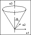
The generating curve of a cone is a line at an angle alpha to the axis of revolution that intersects the axis at the origin. The v parameter is the height of the point along the axis, and the radial distance of the point is v * tan(alpha).
Data Format:
e1[3]      Unit vector, in the u direction
e2[3]      Unit vector, in the v direction
e3[3]      Normal to the plane
origin[3]  Origin of the cone
alpha      Angle between the axis of the cone 
           and the generating line
Parameterization:
(x, y, z) = v * tan(alpha) * [cos(u) * e1 + 
            sin(u) * e2] + v * e3 + origin
Torus
Torus
Image
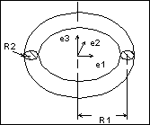
The generating curve of a torus is an arc of radius R2 with its center at a distance R1 from the origin. The starting point of the generating arc is located at a distance R1 + R2 from the origin, in the direction of the first vector of the local coordinate system. The radial distance of a point on the torus is R1 + R2 * cos(v), and the height of the point along the axis of revolution is R2 * sin(v) .
Data Format:
e1[3]      Unit vector, in the u direction
e2[3]      Unit vector, in the v direction
e3[3]      Normal to the plane
origin[3]  Origin of the torus
radius1    Distance from the center of the 
           generating arc to the axis of 
           revolution
radius2    Radius of the generating arc
Parameterization:
(x, y, z) = (R1 + R2 * cos(v)) * [cos(u) * e1 + 
            sin(u) * e2] + R2 * sin(v) * e3 + 
            origin
General Surface of Revolution
Image
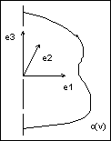
A general surface of revolution is created by rotating a curve entity, usually a spline, around an axis. The curve is evaluated at the normalized parameter v, and the resulting point is rotated around the axis through an angle u. The surface of revolution data structure consists of a local coordinate system and a curve structure.
Data Format:
e1[3]       Unit vector, in the u direction
e2[3]       Unit vector, in the v direction
e3[3]       Normal to the plane
origin[3]   Origin of the surface of revolution
curve       Generating curve
Parameterization:
curve(v) = (c1, c2, c3) is a point on the curve.
(x, y, z) = [c1 * cos(u) - c2 * sin(u)] * e1 + 
            [c1 * sin(u) + c2 * cos(u)] * e2 + 
            c3 * e3 + origin
Ruled Surface
Ruled Surface
Image
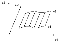
A ruled surface is the surface generated by interpolating linearly between corresponding points of two curve entities. The u coordinate is the normalized parameter at which both curves are evaluated, and the v coordinate is the linear parameter between the two points. The curves are not defined in the local coordinate system of the part, so the resulting point must be transformed by the local coordinate system of the surface.
Data Format:
e1[3]      Unit vector, in the u direction
e2[3]      Unit vector, in the v direction
e3[3]      Normal to the plane
origin[3]  Origin of the ruled surface
curve_1    First generating curve
curve_2    Second generating curve
Parameterization:
(x', y', z') is the point in local coordinates.
(x', y', z') = (1 - v) * C1(u) + v * C2(u)
(x, y, z) = x' * e1 + y' * e2 + z' * e3 + origin
Tabulated Cylinder
Tabulated Cylinder
Image
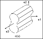
A tabulated cylinder is calculated by projecting a curve linearly through space. The curve is evaluated at the u parameter, and the z coordinate is offset by the v parameter. The resulting point is expressed in local coordinates and must be transformed by the local coordinate system to be expressed in part coordinates.
Data Format:
e1[3]      Unit vector, in the u direction
e2[3]      Unit vector, in the v direction
e3[3]      Normal to the plane
origin[3]  Origin of the tabulated cylinder
curve      Generating curve
Parameterization:
(x', y', z') is the point in local coordinates.
(x', y', z') = C(u) + (0, 0, v)
(x, y, z) = x' * e1 + y' * e2 + z' * e3 + origin
Coons Patch
Coons Patch
Image
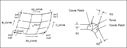
A Coons patch is used to blend surfaces together. For example, you would use a Coons patch at a corner where three fillets (each of a different radius) meet.
Data Format:
le_curve               u = 0 boundary
ri_curve               u = 1 boundary
dn_curve               v = 0 boundary
up_curve               v = 1 boundary
point_matrix[2][2]     Corner points
uvder_matrix[2][2]     Corner mixed derivatives
Fillet Surface
Fillet Surface
Image
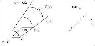
A fillet surface is found where a round or a fillet is placed on a curved edge, or on an edge with non-constant arc radii. On a straight edge, a cylinder would be used to represent the fillet.
Data Format:
pnt_spline   P(v) spline running along the u = 0 boundary
ctr_spline   C(v) spline along the centers of the
             fillet arcs
tan_spline   T(v) spline of unit tangents to the
             axis of the fillet arcs
Parameterization:
R(v) = P(v) - C(v)
(x,y,z) = C(v) + R(v) * cos(u) + T(v) X R(v) * 
          sin(u)
Spline Surface
Spline Surface
Image
The parametric spline surface is a nonuniform bicubic spline surface that passes through a grid with tangent vectors given at each point. The grid is curvilinear in uv space. Use this for bicubic blending between corner points.
Data Format:
u_par_arr[]     Point parameters, in the u
                direction, of size Nu
v_par_arr[]     Point parameters, in the v
                direction, of size Nv
point_arr[][3]  Array of interpolant points, of
                size Nu x Nv
u_tan_arr[][3]  Array of u tangent vectors
                at interpolant points, of size
                Nu x Nv
v_tan_arr[][3]  Array of v tangent vectors at
                interpolant points, of size
                Nu x Nv
uvder_arr[][3]  Array of mixed derivatives at
                interpolant points, of size
                Nu x Nv
Engineering Notes:
•  Allows for a unique 3x3 polynomial around every patch.
•  There is second order continuity across patch boundaries.
•  The point and tangent vectors represent the ordering of an array of [i][j], where u varies with i, and v varies with j. In walking through thepoint_arr[][3], you will find that the innermost variable representing v(j) varies first.
Second Derivative Spline Surface
The Second Derivative Spline Surface (ProSpline2ndDersrfdata) is a bicubic spline surface with possibility of altering the degree of boundary segments to accommodate corresponding curvature (2nd derivatives) conditions. Use this for bicubic blending with second degree derivatives along boundaries.
u_par_arr[]
Point parameters, in the u direction, of size Nu
v_par_arr[]
Point parameters, in the v direction, of size Nv
point_arr[][3]
Array of interpolant points, of size Nu x Nv
u_tan_arr[][3]
Array of u tangent vectors at interpolant points, of size Nu x Nv
v_tan_arr[][3]
Array of v tangent vectors at interpolant points, of size Nu x Nv
uvder_arr[][3]
Array of mixed derivatives at interpolant points, of size Nu x Nv
(*u_der2_arrs[2])[3]
2 Arrays of 2nd U derivatives along V boundaries interpolation points, size of Nv.
(*v_der2_arrs[2])[3]
2 Arrays of 3rd V derivatives along U boundaries interpolation points, size of Nu.
(*uuv_der[2])[3]
2 Arrays of uuv mixed derivatives along V boundaries interpolation points, size of Nv.
(*vvu_der[2])[3]
Arrays of vvu mixed derivatives along U boundaries interpolation points, size of Nv.
der4[4][3] UUVV
derivatives at the corners
Engineering notes:
•  Each second degree derivatives array can be NULL. If it is defined then corresponding 3rd degree mixed derivatives should be defined.
•  Each der4 can be NULL and should be defined if 2nd degree derivatives are defined in both directions at the corresponding corner.
NURBS Surface
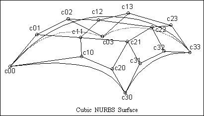
The NURBS (nonuniform rational B-spline) surface is defined by basis functions (in u and v), expandable arrays of knots, weights, and control points.
NURBS Surface
Image
Data Format:
deg[2]             Degree of the basis
                   functions (in u and v)
u_par_arr[]        Array of knots on the 
                   parameter line u
v_par_arr[]        Array of knots on the
                   parameter line v
wghts[]            Array of weights for
                   rational NURBS, otherwise
                   NULL
c_point_arr[][3]   Array of control points
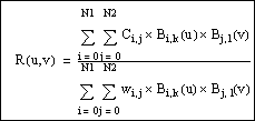
Definition:
Image
k   = degree in u
l   = degree in v
N1  = (number of knots in u) - (degree in u) - 2
N2  = (number of knots in v) - (degree in v) - 2
B = basis function in u
B = basis function in v
w = weights
C = control points (x,y,z) * w
Engineering Notes:
The weights and f arrays represent matrices of size wghts[N1+1][N2+1] and c_points_arr [N1+1] [N2+1]. Elements of the matrices are packed into arrays in row-major order.
Cylindrical Spline Surface
The cylindrical spline surface is a nonuniform bicubic spline surface that passes through a grid with tangent vectors given at each point. The grid is curvilinear in modeling space.
Cylindrical Spline Surface
Image
Data Format:
e1[3]      x' vector of the local coordinate system
e2[3]      y' vector of the local coordinate system
e3[3]      z' vector of the local coordinate system, 
           which corresponds to the axis of revolution 
           of the surface
origin[3]  Origin of the local coordinate system
splsrf     Spline surface data structure
The spline surface data structure contains the following fields:
u_par_arr[]         Point parameters, in the
                    u direction, of size Nu
v_par_arr[]         Point parameters, in the
                    v direction, of size Nv
point_arr[][3]      Array of points, in cylindrical
                    coordinates, of size Nu x Nv. 
                     The array components are as follows:
                     point_arr[i][0] - Radius
                     point_arr[i][1] - Theta
                     point_arr[i][2] - Z
u_tan_arr[][3]       Array of u tangent vectors.
                     in cylindrical coordinates,
                     of size Nu x Nv
v_tan_arr[][3]      Array of v tangent vectors,
                    in cylindrical coordinates,
                    of size Nu x Nv
uvder_arr[][3]      Array of mixed derivatives,
                    in cylindrical coordinates,
                    of size Nu x Nv
Engineering Notes:
If the surface is represented in cylindrical coordinates (r,theta, z), the local coordinate system values (x', y', z') are interpreted as follows:
x' = r cos (theta)
y' = r sin (theta)
z' = z
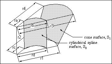
A cylindrical spline surface can be obtained, for example, by creating a smooth rotational blend (shown in the figure).
In some cases, you can replace a cylindrical spline surface with a surface such as a plane, cylinder, or cone. For example, in the figure, the cylindrical spline surface S1 was replaced with a cone
(r1 = r2, and r3 = r4 and r1 r3).
If a replacement cannot be done (such as for the surface S0 in the figure (rarb or rcrd)), leave it as a cylindrical spline surface representation.
Foreign Surface
The foreign surface consists of two perpendicular unit vectors (e1 and e2), the normal to the plane(e3), the origin of the plane and the foreign ID returned by the function user_init_surf().
Data Format:
e1[3]       Unit vector, in the u direction
e2[3]       Unit vector, in the v direction
e3[3]       Normal to the plane
origin[3]   Origin of the plane
foreign_id  Foreign ID returned by user_init_surf()
Parameterization is established by the Foreign Surface callback function user_eval_surf().
Edge and Curve Data Structures
The data structures are used to represent edges (line, arc, and spline) as well as the curves (line, arc, spline, and NURBS) within the surface data structures.
This section describes the edge and curve data structures, arranged in order of complexity. For ease of use, the alphabetical listing of the edge and curve data structures is as follows:
•  Arc
•  Line
•  NURBS
•  Spline
•  Ellipse
Arc
The arc entity is defined by a plane in which the arc lies. The arc is centered at the origin, and is parameterized by the angle of rotation from the first plane unit vector in the direction of the second plane vector. The start and end angle parameters of the arc and the radius are also given. The direction of the arc is counterclockwise if the start angle is less than the end angle, otherwise it is clockwise.
Data Format:
vector1[3]    First vector that defines the
              plane of the arc
vector2[3]    Second vector that defines the
              plane of the arc
origin[3]     Origin that defines the plane
              of the arc
start_angle   Angular parameter of the starting
              point
end_angle     Angular parameter of the ending
              point
radius        Radius of the arc.
Parameterization:
t' (the unnormalized parameter) is 
   (1 - t) * start_angle + t * end_angle
(x, y, z) = radius * [cos(t') * vector1 +
   sin(t') * vector2] + origin
Line
Data Format:
end1[3]   Starting point of the line
end2[3]   Ending point of the line
Parameterization:
(x, y, z) = (1 - t) * end1 + t * end2
NURBS
The NURBS (nonuniform rational B-spline) curve is defined by expandable arrays of knots, weights, and control points.
Cubic NURBS Curve
Image
Data Format:
degree        Degree of the basis function
params[]      Array of knots
weights[]     Array of weights for rational 
              NURBS, otherwise NULL.
c_pnts[][3]   Array of control points
Definition:
Image
k = degree of basis function
N = (number of knots) - (degree) - 2
w = weights
C = control points (x, y, z) * w
B = basis functions
By this equation, the number of control points equals N+1.
Spline
The spline curve entity is a nonuniform cubic spline, defined by a series of three-dimensional points, tangent vectors at each point, and an array of unnormalized spline parameters at each point.
Data Format:
par_arr[]     Array of spline parameters
              (t) at each point.
pnt_arr[][3]  Array of spline interpolant points
tan_arr[][3]  Array of tangent vectors at
              each point
Parameterization:
x, y, and z are a series of unique cubic functions, one per segment, fully determined by the starting and ending points, and tangents of each segment.
Let p_min be the parameter of the first spline point, and p_max be the parameter of the last spline point. Then, t', the unnormalized parameter, is t * p_max + (1-t) * p_min.
Locate the ith spline segment such that:
par_arr[i] < t' < par_arr[i+1]
(If t < 0 or t > +1, use the first or last segment.)
t0 = (t' - par_arr[i])   / (par_arr[i+1] - par_arr[i])
t1 = (par_arr[i+1] - t') / (par_arr[i+1] - par_arr[i])
The coordinates of the points are then:
(x, y, z) = pnt_arr[i] * t1^2 * (1 + 2 * t0) +            
            pnt_arr[i+1] * t0^2 * (1 + 2 * t1) +
          (par_arr[i+1] - par_arr[i]) * t0 * t1 *
               (tan_arr[i] * t1 - tan_arr[i+1] * t0)
Ellipse
Ellipses in 3D geometry is split into two identical half-ellipses. The ellipse is defined by its major and minor axis radius values. Similar to arcs, elliptic segments are defined by a plane in which the ellipse lies, centered at the origin, and parameterized by the angle of rotation. The direction of the ellipse is counterclockwise if the start angle is less than the end angle, otherwise it is clockwise.
Data Format:
center  - Center point of the ellipse
major_axis_unit_vect  - Direction for the X-axis of the ellipse
norm_axis_unit_vect  - Direction for the Y-axis
major_len -  The radiusin the X-direction
minor_leng The radiusin the Y-direction
start_ang The ellipse start angle
end_ang The end angle for the ellipse
The y-axis can be found as a vector product of norm_axis_unit_vect on the major_axis_unit_vect. In actual examples, the major_len can be less than the minor_len.
Parameterization:
t' (the unnormalized parameter) is 
   (1 - t) * start_angle + t * end_angle
(x, y, z) = major_len * [cos(t') * vector1] +
   minor_len * [sin(t') * vector2] + origin
References:
Faux, I.D., M.J. Pratt. Computational Geometry for Design and Manufacture. Ellis Harwood Publishers, 1983.
Mortenson, M.E. Geometric Modeling. John Wiley & Sons, 1985.